PEP 6305 Measurement in
Health & Physical Education
Topic 9: Analysis
of Variance (ANOVA)
Section 9.1
n
This Topic has 2 Sections.
Reading
n
Vincent & Weir, Statistics in Kinesiology, 4th ed. Chapter
11 “Simple
Analysis of Variance: Comparing the Means Among Three or More Sets of Data”
Purpose
n
To demonstrate the comparison of means using analysis of variance
(ANOVA).
The ANOVA Null
Hypothesis and the F Statistic
n
ANOVA compares multiple (≥ 2) means simultaneously. The
purpose is
to determine if the variation among the means is higher than would be expected
by sampling error alone.
n
The ANOVA null hypothesis is that all of the means have the
same value. If the number of means = k , the null hypothesis is:
¨

¨
where μ, the lowercase Greek letter mu, is a symbol
for the population mean.
n
The statistic used in ANOVA is F, which is the ratio of the
variation “between” the groups to the variation “within” the groups.

¨
The observed variance between groups is an estimate of the
variation among the group means in the population. If all groups have the exact
same mean, this variance = 0.
¨
The observed variance within groups is an estimate of the
variation that would be expected to occur as a result of sampling error alone.
¨
If the observed (computed) value for F is
significantly
higher than the value expected by sampling variation alone, then the variance
between groups is larger than would be expected by sampling error alone.
·
In other words, at least one mean differs from the others enough
to cause large variation between the groups.
ANOVA versus t
Test
n
If a
t test compares two means, why not just test each pair
of means instead of using ANOVA? (After all, t tests are easier to do, by
hand anyway, and
easier to interpret, right?)
n
Performing multiple t tests
in one set of data causes a number of problems.
¨
Increases the type I error probability (α): If you
conduct multiple tests in a single set of data, you are compounding error
probability and increasing the chance of rejecting the null hypothesis when
it is actually true (a
type I
error). (See
here for an explanation.)
¨
Does not use all of the available information: t
tests compare only two means, using an estimate of sampling error from the two
groups being compared. ANOVA uses an estimate of sampling error from all groups.
Recall from the
Central Limit Theorem that sampling error decreases as sample size increases; thus, the ANOVA
estimate of sampling error is typically more accurate than the estimates from
t tests.
¨
Increases time and effort: Obviously, doing more
tests take more time and you have to read more computer output. While this is
not a tremendous concern if there are 3 or 4 groups, in complex studies the
number of paired comparisons can be very large.
¨
Does not allow testing of complex hypotheses:
Vincent does not mention this limitation, but it is important. In complex
studies, we often have hypotheses about whether one factor influences the way
that another factor influences the dependent variable. Using t tests to
compare group means cannot answer these questions, meaning that you have not
tested your hypothesis. The flexibility of ANOVA allows for testing these
types of hypotheses directly.
n
ANOVA indicates whether one or more means differs from the others;
it does not tell you which means differ from one another.
¨
Techniques known as post hoc (Latin for “after the fact”)
tests
are used to identify which means differ. Post hoc tests are discussed
in the next section.
ANOVA Assumptions
n
Normality
¨
The dependent variable is
normally distributed in the population
being sampled.
¨
This assumption is needed to interpret
variance properly.
¨
Normality of the dependent variable can be evaluated using a
histogram and
skewness
and kurtosis statistics.
¨
ANOVA, however, is remarkably accurate ("robust") even if this
assumption is not met.
n
Homogeneity of variance
¨
This means that the variances within each group are equal in the population being
sampled.
¨
This assumption is needed to allow for computing a pooled
(combined across all groups, sort of like an average) estimate of sampling
variance. If one or more groups had a variance that was much larger or much
smaller than the other groups, the “average” variance would be inaccurate (not
representative of the population) for any of the groups (too large for some, too
small for others). Since sampling variance is used to compute the F statistic,
if the estimate of sampling variance is inaccurate, the accuracy of the F test
is questionable.
¨
Homogeneity of variance can be evaluated using a variety of
statistical tests, but the most straightforward method is to compare the
within-group variances; one or more variances twice as large as other variances
may be a problem.
¨
This assumption affects ANOVA more than normality, but only large
differences in the variances (i.e., one twice as large as another) produce a noticeable effect.
n
Independence 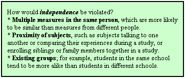
¨
This means that the scores are not affected by other scores, which means that
subjects in one group did not influence subjects in other groups.
¨
This assumption is needed to allow for computing the variance
between groups. If one group influences scores in another group, then comparing
scores between those two groups is biased—one group will always have higher or
lower scores regardless of any treatment effect being present.
¨
Random sampling, random assignment to groups, and keeping the
groups separated during the study ensures
independence.
¨
This assumption is critical; violation invalidates the results.
¨
Repeated measures analyses (see
Topic 10) are used when scores are
not independent.
“Between”
Variance and “Within” Variance
n
Group means are computed within each group by summing the
scores in that group and dividing by the number of subjects in that group:
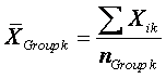 where Xik is the score of a person (i) in group k
and nGroup k is the number of subjects in group k.
where Xik is the score of a person (i) in group k
and nGroup k is the number of subjects in group k.
n
A "grand" mean is computed across all groups by summing
the scores of all subjects across all groups:
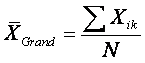 where N is the total number of subjects in the study (the sum of all nGroup).
n
The between group variance is the variation of the group
means from the grand mean.
n
The within group variance is the variation of each subject
from the group mean of the group to which they belong.
n
The total variance is the variation of each subject from
the grand mean (the sample variance computed in Topic 4).
n
These three variance are related: VarianceTotal =
VarianceBetween + VarianceWithin
Sum of Squares
n
A sum of squares (SS) is the sum of the squared
deviations. 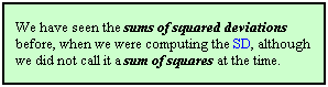
n
Each component (Between, Within, and Total) in ANOVA has a SS.
¨
Between SS:  ,
summing across all k groups, multiplying by n in each group to
make SSB comparable to SSWithin and SSTotal
; this multiplication equalizes the scale of the SS values.
,
summing across all k groups, multiplying by n in each group to
make SSB comparable to SSWithin and SSTotal
; this multiplication equalizes the scale of the SS values.
¨
Within SS:  ,
summing across the nGroup subjects in each group, then across
all k groups, which means you are summing across (nGroup
× k) = all N subjects.
,
summing across the nGroup subjects in each group, then across
all k groups, which means you are summing across (nGroup
× k) = all N subjects.
¨
Total SS: 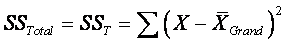 ,
summing across all N subjects.
,
summing across all N subjects.
n
Each of these SS is a measure of
variability.
n
ANOVA compares the between-groups variability with the
within-groups variability using the F statistic.
n
Because the SS depend on the number of elements being summed, and
the number of elements for the Between SS is less than Within SS (you have fewer
groups than you have subjects), then both SS measures are standardized by their respective
degrees of freedom, creating Mean Squares.
Mean Squares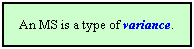 and the F Statistic
n
A mean square (MS) is the mean of a series of
squared deviations.
n
A MS is computed by dividing a SS by its
degrees of freedom
(df).
¨
df = (the number of elements being summed in the SS) – (the
number of means subtracted in the SS)
¨
For each SS equation, compute the difference between the number of
elements ahead of the subtraction sign from the number of elements behind the
subtraction sign.
¨
dfBetween : How many elements are being summed in the SSB
equation above? The k group means. How many means are subtracted from
these k elements? One—the grand mean is subtracted from all k group
means. So dfB = k – 1.
¨
dfWithin : How many elements are being summed in the SSW
equation above? The (nGroup × k groups) = N subjects.
How many means are subtracted from these N elements? The k group means
are subtracted from the n subjects in each group. So dfW = N –
k.
¨
dfT : What is the df for SSTotal?
Note that dfT = dfB + dfW = (k – 1) + (N – k) =
k – 1 + N – k = N – 1 .
n
Divide each SS by its df to find the corresponding MS.
¨
Between: 
¨
Within: 
n
FINALLY, we compute F :
 MSW represents the variation expected as a result of sampling
error alone.
MSW represents the variation expected as a result of sampling
error alone.
n
The
sampling distribution of F in the population is known,
so we can compare our observed sample F value to the distribution to
determine the error probability for the observed value.
¨
If MSB is several times larger than MSW,
we may conclude that the variation between groups is significantly larger than sampling error.
n
MSW is often called mean square error (MSE),
referring to sampling error. MSW and MSE
are exactly the same thing.
 Click
to go to the next section (Section 9.2)
Click
to go to the next section (Section 9.2)