PEP 6305 Measurement in Health & Physical Education

Topic 4: Measures of Variability

Section 4.1

n   This Topic has 1 Section.

Reading

n   Vincent & Weir, Statistics in Kinesiology 4th ed., Chapter 5 “Measures of Variability”

Purpose

n   To discuss and demonstrate various measures of variability in a distribution of scores.

Variability

n   Variability is an indicator of how widely scores are dispersed around the measure of central tendency.

¨  Example: the GRE quantitative and verbal sections range from a high score of 800 to a low score of 200. This spread of scores is one indicator of the variability of GRE scores.

¨  Does a leptokurtic or platykurtic distribution have a larger relative variability about the central score? Can you sketch a line drawing of these distributions that shows why?

n   A distribution is described by both its central value and its variability.

¨  Reporting both measures is necessary to characterize the distribution of data appropriately.

¨  When central tendency and variability are known, different sets of data can be compared—which is a big deal in statistics.

n   Generally, four indicators of variability are used: range, interquartile range, variance, and standard deviation.

Range                                                       

n   The range is the difference between the highest and lowest scores.

¨  The picture at the right shows the tallest (7' 6" Yao Ming) and shortest (5' 5" Earl Boykins) NBA professional basketball players from the year 2006.

¨  The range of heights of NBA players in 2006 was therefore 90 inches - 65 inches = 25 inches, or 2 feet 1 inch (looks like more than that, doesn't it?).

n   The range can change dramatically with a change in either the highest or lowest value (what would the range be if Boykins was released in mid-season and the second shortest player was 5' 10"? Answer).

n   The range is thus not a stable measure of variability, but can give a rough indication of how scores are dispersed.

Interquartile Range                                  

n   The interquartile range is the difference between the scores at the 75^th and 25^th percentiles (top of Q3 – top of Q1). Half of the scores in the distribution lie in the interquartile range. (Why?)

n   The interquartile range is more stable than the range because the extreme values (highest and lowest) are not part of its computation. Thus, the extreme values can change by very large amounts, but the interquartile range will likely be unaffected.

n   The interquartile range is used for ordinal data, or to describe the variability of highly skewed interval or ratio data (Why?).

Population Variance

n   The variance uses deviations (d), or the difference between each score and the mean, to compute an indicator of variability.

¨  The idea is that all of the d's can be combined to compute the average deviation; the average distance between the mean and the scores.

n   The sum of the deviations for any set of data is 0 (∑d = 0; see Table 5.1). So we cannot use the sum of the deviations as an indicator of variability.

n   Instead, we sum the squares of the deviations; this takes care of the “sum to zero” problem, because the sum of the squared deviations will not sum to 0 (∑d² > 0).

n   To normalize the sum of squared deviations ( ∑d² ), divide by the number of scores (N). The resulting value is the variance (V):

          The variance may also be symbolized by σ² (population parameter). [σ is the lowercase Greek letter sigma]

Population Standard Deviation (Parameter)

n   The measurement unit for variance is the squared measurement unit of the original variable. This makes it difficult to interpret and compare between variables; it would be easier if the indicator of variability was in the same unit as the original variable.

n   The solution is easy enough: take the square root of the variance.

n   This value is called the standard deviation (σ) because it is the average deviation in the same unit as the original variable; this is what we set out to find.

n   This formula can be unwieldy in large data sets, so a user-friendly formula is provided that requires only the square of each score and the mean:

n   Of course, you would just use a computer to calculate the standard deviation, right? Yes—except that statistical programs compute a sample standard deviation, not the population parameter standard deviation.

¨  If for some reason you have all of the data in the population, you would use one of the formulas above to calculate the parameter value.

¨  This would be very unusual. In the vast majority of cases you would be interested in computing the…

Sample Standard Deviation (Statistic)

n   When a sample is used to calculate a value rather than using the entire population, it always underestimates the population value. Thus, the formula for computing the sample standard deviation has a built-in adjustment to account for the underestimation. 

n   The adjustment brings attention to a very important statistical concept: degrees of freedom (df). The “degrees” part means a number that is a count of something (subjects, groups, etc.). The “freedom” part means the number of values in the data that are “free to vary.”

¨  Free to vary means that when one statistic is calculated using another statistic, the amount of information used to make the calculation is limited--you have less information for the second statistic than you did for the first because you used some of that information in computing the first statistic.

¨  So, since the sample standard deviation (a statistic) uses the sample mean (also a statistic) in its calculation, the information is limited. The information is limited because you have used some of the information in the data to estimate the mean.

¨  The example given on page 65 of the text demonstrates the df concept. If there are four scores, and the computed (sample) mean is 5, then (using the formula for computing the mean) the sum of the four scores must be 20. Why?

     ¨  Recall from Topic 3, the formula for the mean:       . 

¨  If you rearrange the terms, the sum ( ∑ X )  =  .  So: Sum = 5 (mean) x 4 (N) = 20.

¨  What this means is that if both N and  of a sample is known then the sum is determined (i.e., known).

¨  Consequently, if you know the sum of four values, and you know any three of the values, then the fourth value is “not free to vary.”

     ¨  Thus, there are only 3 “degrees of freedom” in this example.

n   The adjustment to the formula for the sample standard deviation (SD) involves dividing the sum of the squared deviations by the degrees of freedom, which is the sample size (N) minus 1 (you subtract 1 because you used that information to compute the mean):

    Definitional formula:      , and computational formula: 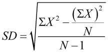(the computational formula is easier when computing by hand, because all you need is the sum of the scores and the sample size).   

n   As stated above, you would usually use a computer program such as R Commander to calculate the SD.

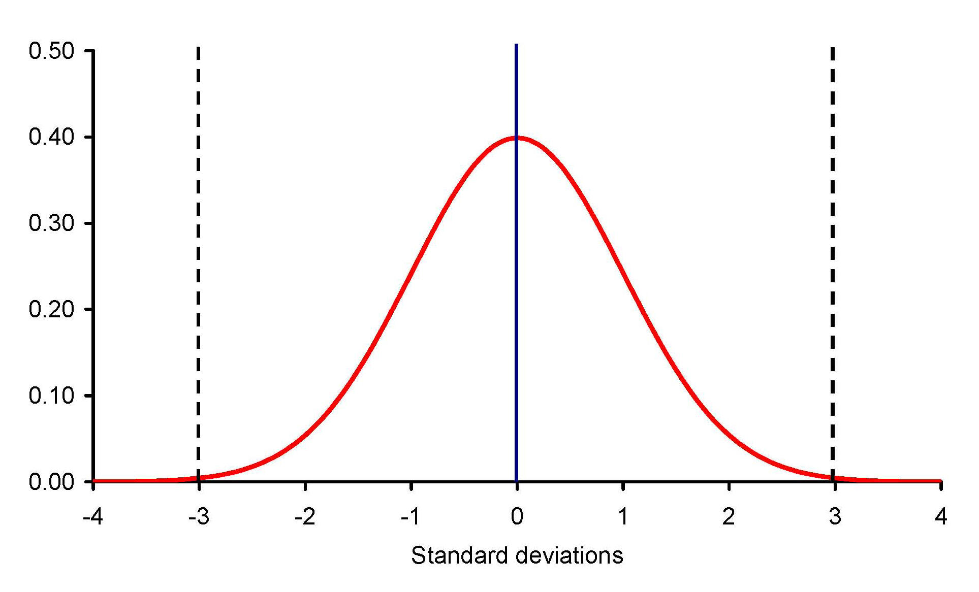
n   In a normal distribution, there are about 3 SD between the mean and the highest score, and about 3 SD between the mean and the lowest score, for a total dispersion (range) of scores of about 6 SD, as shown in this figure:

n   Most of the values in the normal distribution (under the red curve) are within ±3 SD of the mean (the blue line at SD = 0). Very few scores exist beyond 3 SD on either side of the mean.

n   In the next Topic, we will discuss how to use the standard deviation and its relation to the normal distribution.

Formative Evaluation

n   Compute by hand the SD for these by-now familiar data: 525, 505, 507, 654, 631, 281, 771, 575, 485, 626, 780, 626. What is the range of these data? What is the interquartile range? (Answers) 

¨  Compute the SD using R Commander. Enter the data in a blank New data set. Go to Statistics>Summaries>Numerical summaries… Click to highlight the variable in the Variables box, click OK. An output file shows the mean, SD, and quantile values.

¨  Your hand-computed values and R Commander values for mean and SD should be the same.

n   Open your data file in R Commander and compute the mean and SD of age, ht (height in cm), wt (weight in kg), bmi (body mass index), pfat (% body fat), and afit (aerobic fitness). What is the median and range of each variable?

n   Tables are an efficient way to present descriptive data. Make a table summarizing your the data in your data file. Put the names and units of measurement for the variables in the left column. In the top row, put the name of the statistic being reported. Tables should be numbered, even if there is only one table, and should have a title. Your final table should look something like this (except with your data file's actual numbers):

Table 1. Characteristics of the study sample (n = 1000).

SD = standard deviation.

BMI = body mass index.

n   In other types of tables, the columns might represent groups of subjects or time intervals (before and after, for example). Alternately, a table can have one or two of the independent variable as rows and the other variables in the columns.

You have reached the end of Topic 4.

Make sure to work through the Formative Evaluation above and the textbook problems (end of the chapter). (remember how to enter data into R Commander?)

You must complete the review quiz (in the Quizzes folder on the Blackboard course home page) before you can advance to the next topic.