PEP 6305 Measurement in
Health & Physical Education
Topic 9: Analysis
of Variance (ANOVA)
Section 9.2
 Click to go to
back to the previous section (Section 9.1)
Click to go to
back to the previous section (Section 9.1)
Example:
Calculating F
n
Vincent provides two methods to calculate F for ANOVA.
¨
We will review the definitional formula method because it
demonstrates the computation of SS and MS explicitly. While it is more tedious,
I think it communicates the concept of ANOVA more clearly.
¨
We will not review the raw score method because you will (if you
are lucky)
never calculate ANOVA by hand--you will use a computer like everyone else does.
¨
In the next section, we will also review how to do simple ANOVA in
R Commander. (You'll use R Commander to complete the assignment and exam).
n
These are the data from Table 11.1 in the text, comparing four
strength training methods (X1 to X4) to a control group:

n
The null hypothesis is that all of the training methods are
equivalent. What is the
research hypothesis?
n
The first step is calculating the means of each group (shown
in the table above), and the grand mean (5.77).
n
Second, calculate MSB.
¨
SSB = nGroup × ∑(XGroup
– XGrand)2 = 7 × [(5.29 – 5.77)2 + (7.86
– 5.77)2 + (5.00 – 5.77)2 + (6.29 – 5.77)2 +
(4.43 – 5.77)2] = 7 × 7.26 = 50.82
¨
dfB = (5 – 1) = 4
¨
MSB = 50.74 / 4 = 12.69 (note: these numbers are
slightly different from the text because I rounded to 4 decimal places, whereas
Vincent & Weir round to 2 places)
n
Third, calculate MSW.
¨
SSW = ∑∑(X – XGroup)2
= 47.43 (see Tables 11.2 and 11.3 for the differences between each score and the
grand mean)
¨
dfB = (35 – 5) = 30
¨
MSW = 47.43 / 30 = 1.58
n
Fourth, compute F.
¨
F = MSB / MSW = 12.69 /
1.58 = 8.02 (again, this is slightly different from the text due to rounding
differences)
n
So, we
have an observed F value. Now what?
The F Test
n
F is a
statistic that has a
known sampling distribution
(the F distribution is named after a
famous statistician named R.A. Fisher).
n
The F test is the comparison of an
observed value of F
to the appropriate known F distribution.
n
In ANOVA, the observed sample F is compared to the
appropriate F distribution to evaluate the error probability of the
observed value.
n
The F distribution has two df; one for the numerator (MSB)
and one for the denominator (MSW).
¨
This makes tables of F extensive and tedious to read (see
Tables A.4, A.5, and A.6).
n
Fortunately, statistics programs compute the type I error
probability when you run ANOVA, so you have no need for consulting tables.
n
In addition, most statistical programs and many spreadsheet
programs such as Excel have functions for
the F distribution programmed into the software, which makes obtaining
the type I error probability (the p-value) simple.
n
For the example above, the observed F value is 8.02, with df = (4,
30) (df numerator = 4, df denominator = 30).
¨
In Excel, the function is FDIST. Open Excel, click in a cell, and click the
fx symbol next to the formula bar (at the top of the data grid).
¨
From the drop-down “Or select a category” menu, select
“Statistical,” then scroll down to select FDIST and click OK.
¨
Enter X = 8.02, Deg_freedom1 (numerator) = 4, and Deg_freedom2
(denominator) = 30. The function returns the p value, in this case 0.00016,
which you would report as “p < 0.001”.
¨
We conclude that at least one of the means differs from the others
by a “significant” amount.
n
Computer output for an ANOVA F test typically includes an
ANOVA table with the source of variance (Between Groups, Within
Groups, etc.), SS, df, MS, F,
and p values.
n
The content of this table is fairly standard output regardless of
the statistics program used, although the layout may differ slightly:

n
For the example above from Vincent & Weir, using the information
we computed, the ANOVA table is:

n
Notice this is the same result that you obtained using hand calcualations and Excel.
ANOVA in R
Commander
n
Single-factor ANOVA (one grouping factor, as in the
example) is relatively straightforward in R Commander, even though we're using
command lines (programming text) rather than point-and-click menus.
n
R
Commander
¨
Download
the
'Table11.1' data file from Blackboard,
or right-click
and "Save target as..." to download and save the
Table11_1.RData file to your drive.
Open R Commander and load the data set. Click the "View data set" button in
R Commander and note that the data are entered in a Data file in
three columns
instead of the five columns shown in Table 11.1.
¨
In the first column is a variable called “subid” (subject
identification) with a different number for each subject.
¨
In the second column is a variable called “group” with a code
letter for each group. There are 5 groups: Group A, Group B, Group C, Group
D, and Group E.
¨
In the third
column is a variable called “score” that contains the scores shown in Table 11.1
in the book.
¨
There are a total of 35
rows (5 groups x 7 subjects/group), one row for each subject. (We'll see in the
repeated measures Topic that sometimes the subjects each have data in more
than one row.)
¨
You'll need the
ez
package
in R to do your ANOVAs and repeated measures ANOVA (next Topic).
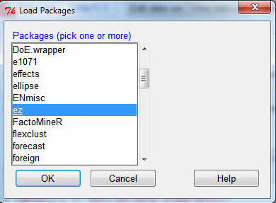
Go to Tools>Load packages...
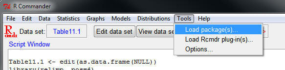
...and in the Load Packages dialog box, scroll down and select 'ez'.
Click OK. (you downloaded
the 'ez'
package at the start of the semester; if you don't see
ez in the list, you didn't, so do it now)
¨
You'll see the phrase library(ez, pos=4) in
your Script and Output windows when the ez
package has loaded.
¨
The ez package
has a number of different functions and tests. The function we're interested in
for this course is
ezANOVA
(see p. 5 of the
ez
PDF).
¨
Here is the command you'll type in the R
Commander Script Window to do the ANOVA described above:
ezANOVA(data=Table11.1, dv=.(score), wid=.(subid), between=.(group),
detailed=TRUE)
¨
What does all of that mean? ezANOVA
is the name of the program, and the rest in the parantheses is the program
input/information that the program needs to run the analysis. R programs run by
naming a program and enclosing the needed information in parantheses. The
ezANOVA program needs the following information
for one-way (between-subjects) ANOVA:
¨
data=Table11.1
tells the program to use the Table11.1 dataset.
¨
dv=.(score)
tells the program that the dependent variable (dv)
is a variable called 'score';
you put a period and parantheses to identify the word as a variable to the
program.
¨
wid=.(subid)
tells the program which variable (subid)
that identifies the subjects; wid
stands for "within ID", meaning within-subjects identifier. (This will be
particularly important for repeated measures ANOVA.)
¨
between=.(group) tells the
program which variable (group)
identifies the groups; group is a between-subjects factor because each
subject is a member of one and only one group.
¨
detailed=TRUE
tells the program to print out a little more information
than the default output, including the SS values.
¨
Once you've typed in the command shown above, click the Submit button to the
lower right of the Script Window, and you should see some Output:
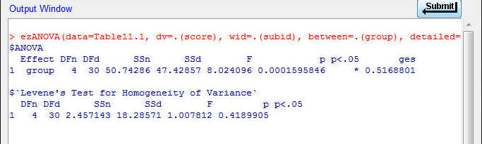
¨
The output under the $ANOVA
label shows the ANOVA table.
It lists the effect (group, which is the only effect in this ANOVA), the degrees
of freedom (DF) for the numerator (DFn) and denominator (DFd), the SS for the
numerateor (SSn) and denominator (SSd), the F ratio, the p-value for the test of
the F ratio, an asterisk in the 'p<.05' column indicating the p-value is
statistically significant, and the effect size (generalized eta squared, ges,
see below).
¨
Although the layout is somewhat different, this is
the same ANOVA table shown above for the Table 11.1 data (within rounding error).
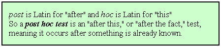
Post Hoc
Tests
 n
Post hoc tests identify which means
differ from one another.
n
Post hoc tests identify which means
differ from one another.
n
They are performed after the ANOVA F test indicates that
significant differences exist among the means.
¨
If the F test is not significant, post hoc tests are
not needed (because none of the means differs from the others.
n
The key advantage of post hoc tests is that some of them
make adjustments to
limit the compounding of type I error probability,
as would occur when using multiple unadjusted t tests to compare means
after a significant ANOVA F test.
Scheffé Interval
n
The post hoc Scheffé test allows for comparisons of not
only each mean to
each of the other means, and allows for comparison of combinations of means to single
means or to other combinations of means.
n
The test computes the smallest interval, or difference between
means or combinations of means,
that would be statistically significant.
¨
The difference for any comparison that exceeds this minimum value
is unlikely to be a result of sampling error alone.
n
The interval (IScheffé) is computed using the
following formula:
 where
k is the total number of groups, Fα is the critical
F value for the specified α type I error level, MSE is the
mean square error (within) term from the ANOVA table, and n1
and n2 are the number of subjects in each of the groups (or
combination of groups) being compared.
where
k is the total number of groups, Fα is the critical
F value for the specified α type I error level, MSE is the
mean square error (within) term from the ANOVA table, and n1
and n2 are the number of subjects in each of the groups (or
combination of groups) being compared.
n
Enter the information from the Table 9.1 example above for α = 0.05; you
should find the minimum statistically significant difference between means is
2.20.
Tukey HSD
n
If you are only comparing group means, and not
comparing any combinations of means, Scheffé provides an interval that is
slightly too
large.
n
A test called Tukey’s Honestly Significant Difference (HSD)
provides a slightly smaller interval:
 where
terms are defined as in Scheffé, except for the q term. q is the
Studentized Range statistic, which is provided in tables in the back of
the text. q is distributed according to the number of groups (k)
and the df of MSE from the ANOVA table.
where
terms are defined as in Scheffé, except for the q term. q is the
Studentized Range statistic, which is provided in tables in the back of
the text. q is distributed according to the number of groups (k)
and the df of MSE from the ANOVA table.
n
Fortunately (for you and me), both the Scheffé interval and the
Tukey HSD (and a number of other post hoc tests) are included in the LazStats
One-way ANOVA procedure (on the main menu window, to the right), so
you don’t have to calculate them by hand.
n
As shown on page 191 of the text, bar graphs are often a good way
to show comparisons of means.
n
The importance of evaluating
effect size
was discussed in
Topic 8.
n
Two measures of effect size can be reported for ANOVA: R2
and omega squared (ω2).
n
R2 is the
squared correlation coefficient, and
the same effect size measure of proportion of variance described in Topic 8.
¨
The proportion of variance aspect is most evident in the R2
formula:
 As can be seen, R2 is the ratio of variation due to
groups to the total variation in the sample.
As can be seen, R2 is the ratio of variation due to
groups to the total variation in the sample.
¨
In ANOVA, R2 is called eta squared (η2)
(lowercase Greek letter eta = η), to distinguish it from the R2
value in regression analysis, although both are interpreted in the same
way.
¨
In the R ezANOVA
program, as described above, a generalized eta squared (η2) is reported
in the Output in the column labeled 'ges'.
n
ω2 (omega squared) is also a measure of
proportion of variance, but it is corrected for sampling error and thus is more
representative of the effect size in the population.
¨
The ω2 formula is a little more complicated:
 In this formula, ω2 is the ratio of variation due to
groups plus sampling error to the total variation plus sampling error.
The variable k is (still) the number of groups.
In this formula, ω2 is the ratio of variation due to
groups plus sampling error to the total variation plus sampling error.
The variable k is (still) the number of groups.
¨
The inclusion of the MSE term provides the
adjustment for inferring that the magnitude of the association is a certain size
in the population.
¨
ω2 is not provided by
ezANOVA, but can be easily computed
using the SS and MS in the ANOVA table.
Formative
Evaluation
n
Use R Commander and ezANOVA to
work problems 1, 2, and 3 at the end of the chapter.
You have reached the end of Topic 9.
Make sure to work through the Formative Evaluation
above and the textbook problems (end of the chapter).
(remember how to enter data into R Commander?)
You must complete the review quiz (in the Quizzes
folder on the Blackboard course home page) before you can advance to the next topic.