PEP 6305 Measurement in Health & Physical Education

Topic 6: Correlation

Section 6.2

Click to go to back to the previous section (Section 6.1)

Calculating the Correlation Coefficient    

n   Similar to the mean and SD, there are several formulas for computing a correlation coefficient.

n   The definitional formula reveals the concept of product moment correlation (which is symbolized by r): 

n   This formula shows that the correlation coefficient is a function of a “product moment,” or the average of the product of two Z scores.

n   A few things about the magnitude and direction of the correlation coefficient can be noted from this definitional formula:

¨  The product of two positive numbers is positive; the product of two negative numbers is also positive. The average of a set of positive numbers is a positive number. This occurs when subjects have generally either positive or negative Z scores on BOTH variables, which means that the direction of the correlation will be positive (direct).

¨  The product of a positive number and a negative number is negative. The average of a set of negative numbers is a negative number. This occurs when subjects have generally a positive Z scores on one variable and a negative Z score on the other variable, which means that the direction of the correlation will be negative (inverse).

¨  If a third of the subjects have positive-positive paired Z scores, a third have negative-negative paired Z scores, and a third have positive-negative paired Z scores, then the average of the products of these values will tend to be close to 0, which has no magnitude and no direction (since 0 has no magnitude and is neither positive nor negative). Such variables would be uncorrelated (r = 0).

¨  This Excel file (click here) shows these relations governing the correlation coefficient.

n   The textbook gives a "machine" formula for computing a correlation coefficient (pp. 113). If you plan to compute by hand, that equation may be of use to you. I always use a computer, and you will use a computer for the assignments and exams in this class (unless you actually want to do it by hand...!!).

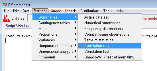
n   Open R Commander and load Dataset6305. Go to Statistics>Summaries>Correlation matrix…

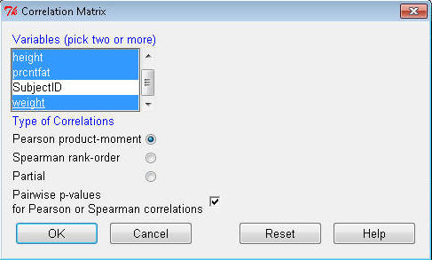
¨  Click to highlight age, height, weight, bmi, prcntfat, and aerobfit (hold the Control key to select multiple variables). Check the "Pairwise p-values..." box as shown. Click OK.

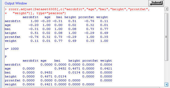
¨  The Output window first shows you a correlation table. The correlation coefficients between each pair of variables is provided, as well as the sample size (n = 1000). You'll notice that the values on the diagonal of the table are all 1.00, since the correlation of a variable with itself has to be 1.00.

¨  The next table in that window, labeled 'P', shows the respective error probability.  

¨  Interpreting these results, the correlation coefficient for weight and age (r = 0.01) has a probability of p = 0.6421 (64.2%, or 64.2/100) of being a result of sampling error alone. From these results we conclude that weight and age are uncorrelated, because the correlation value has a good chance of simply being a result of sampling error.

¨  By contrast, the correlation coefficient for height and weight (r = 0.69) has a probability of p = 0.0000, or p < 0.001 (less than 0.01%, or 1/10,000) of being a result of sampling error alone. We conclude that height and weight are significantly correlated because that value would be highly unlikely if the variables were actually uncorrelated.

¨  Examine the values in this table and identify which associations are statistically significant (p ≤ 0.05).

Interpreting the Correlation Coefficient

n   The interpretation of the magnitude of the correlation coefficient can be a little tricky. The same magnitude correlation coefficient may represent a large and important association in some circumstances but a relatively meaningless relation in other circumstances.

n   In general, there are two considerations when evaluating the magnitude of the correlation coefficient.

n   First, evaluate how much of the variation in one variable "overlaps" with variation in the other variable, which is measured by the square of the correlation coefficient (r² or R²), known as the “proportion of common variance.” This is the proportion of variation in one variable that can be accounted for by variation in the other variable.

¨  In general, as correlation coefficients get larger than 0.33 (r² ≥ 0.10) they are more likely to be important.

¨  But the importance of magnitude differs from field to field and study to study. It is best to determine what size correlation would be meaningful in a practical sense (i.e., provide a meaningful explanation) before collecting and analyzing the data.

n   Second, determine whether the correlation coefficient is significantly different from 0, which would mean that the observed correlation was unlikely to have occurred by chance (as we did in the correlation table above).

¨  To be able to interpret the statistical significance of the correlation coefficient, the study has to be designed properly, with an appropriate sample size and data collection strategy.

¨  Sample size is a key issue because larger sample sizes allow correlation coefficients with smaller magnitudes to be shown to be significantly different from 0. Appendix Table A.2 in the text shows this relationship; degrees of freedom = N – 2 (why?), so you can see how fewer subjects requires a larger correlation coefficient for the significance test.

¨  For example, for an error probability of α = 0.05 (the third column) and n = 14 subjects, so the degrees of freedom is df = n - 2 = 14 - 2 = 12 a correlation coefficient of 0.532 or higher occurs fewer than 5 times out of 100 by chance alone. By contrast, if you have 32 subjects (df = 30), the correlation coefficient with the same error probability is 0.349.

n   So, if the correlation coefficient is large enough and is significantly different from 0, the correlation coefficient probably indicates an important relationship exists between the variables.

n   Recall that correlation does not imply causality. A very large magnitude correlation coefficient that is statistically significant may be describing an association with no cause-and-effect relation between the two variables.

¨  For example, age is highly correlated with risk of skin cancer, but one does not "cause" the other. Both are related to a third variable, total (lifetime) exposure to ultraviolet radiation—the older you are, the more UV exposure you've had, and the more UV exposure you've had, the higher the risk of skin cancer. Age by itself does not cause skin cancer, and skin cancer does not "cause" aging.

Formative Evaluation

n   Work through the R Commander examples in the lecture notes above.

n   Work problems 1, 2, and 4 at the end of Chapter 7. (Use a computer program to do the statistics questions).

n   In your own field of interest in HHP (nutrition, exercise science, sports administration, or health), name two variables that are likely to be positively correlated.

n   In your own field of interest in HHP, name two variables that are likely to be negatively correlated?

You have reached the end of Topic 6.

Make sure to work through the Formative Evaluation above and the textbook problems stated above (end of the chapter). (remember how to enter data into R Commander?)

You must complete the review quiz (in the Quizzes folder on the Blackboard course home page) before you can advance to the next topic.