PEP 6305 Measurement in
Health & Physical Education
Topic 5: The
Normal Distribution
Section 5.2
 Click to go to
back to the previous section (Section 5.1)
Click to go to
back to the previous section (Section 5.1)
Statistical
Inference: Estimating Parameters
n
We usually cannot measure and evaluate an entire population. For
example, if we want to know the population average body composition and its variability in American adults, we would have to measure over 200 million people!
Clearly, that is impractical. 
n
When evaluating the population is impractical (as is nearly always
true), a sample of
the population is evaluated to obtain an estimate of the parameter
(i.e., estimate the population value).
n
Sampling and inference were briefly introduced in
Topic 1.
Sampling Error
n
One limitation of using a statistic to estimate a parameter is that
the statistic is unlikely to be exactly equal to the parameter.
¨
The sample may have a few too many subjects with high scores or a few too many subjects with low scores.
¨
As a result, the value of the statistic may be slightly higher
or slightly lower than the true population value.
n
Sampling error is the variation in the statistic value
(too high or too low) relative to the true parameter value.
Sampling error is
deviation from the population value that results from using a sample (part of
the population) instead of
the entire population.

¨
Sampling error is used to evaluate the accuracy of a statistical
estimate of the parameter value.
¨
The larger the sample size, the smaller the sampling error. See
this graphic example in Excel.
n
Suppose that
a statistical value (such as the mean) was
computed in a large number of different samples that were all selected from the
same population. As the size of each sample
gets larger, the values of the computed statistic becomes more normally distributed.
¨
This concept is called the central
limit theorem, which implies that as the size of the sample increases, the
distribution of the statistic (not the distribution of the variable, but
of the
statistic that is computed, such as the mean) becomes normally distributed,
with a mean equal to the population value. (You can download a small program
that graphically demonstrates this
here.)
¨
For example, if you computed the mean in 50 different samples of
the same size,
a frequency histogram of those 50 means would be normally distributed.
¨
The mean of that distribution of 50 means is the "mean of the
means"; this value is a good approximation of the actual population mean.
¨
The distribution of the 50 means also has a standard
deviation (SD), which could be called the "SD of the means"
(note that this is not the same as the SD in each sample);
to distinguish this statistic from the sample SD, this value is called the
(SEM).
¨
The formula for the SEM is:
 The
SEM
can be computed using the SD and N from a single sample,
without collecting 50 (or more) samples!
The
SEM
can be computed using the SD and N from a single sample,
without collecting 50 (or more) samples!
Example
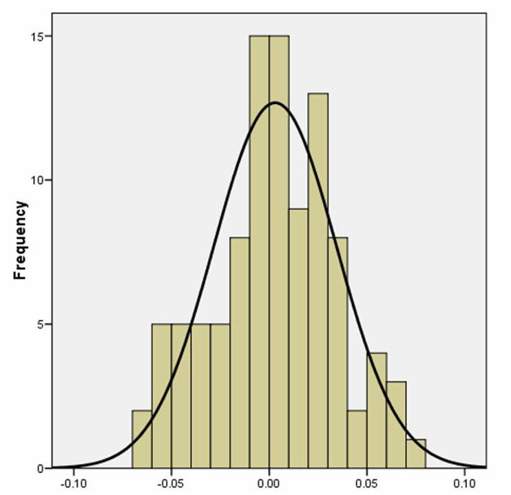
The histogram at right shows an example of the distribution of 100 means computed from samples of randomly generated data. Each sample had 1000 values (N = 1000). The mean of the variable
in the "population" I used to create the 100 samples was 0 and the SD was 1.0
(I know those are the values because I created them!). Since the
data were randomly generated, however, each sample's mean and sample SD varied
slightly from these values.
The "mean of these means" of these 100 samples is
0.003, which is close to 0, the
population parameter value.
The SEM,
or "SD of these means," was computed to be 0.0315.
If we took only one of these samples of N = 1000 and computed the SEM,
the estimated SEM value would be SD/√n = 1.00/√(1000) = 1/31.623 = 0.0316,
which is extremely close to the 0.0315 value actually calculated from the 100 samples.
This example shows that we we can be confident that our statistical results are
reasonable estimates of the population values.
n
The SEM can be used to estimate a range of values in
which the true population mean is likely to be.
¨
Recall that approximately 68% of the scores in a normal
distribution are within ±1 SD, as discussed in
Section 5.1.
(Recall the relation between the SD
[Z scores] and percentiles in the normal
distribution?)
¨
When the mean is estimated from sample data, you can say that the population mean
is within ±1 SEM of the sample mean with "68% confidence".
¨
“Confidence” means that if a large number (>100) of
additional random samples of the same population were collected under the same conditions and the mean and SEM
were computed for each of those 100 samples, then 68% of the ±1 SEM
ranges (the SEM ranges are called "confidence intervals") would include the actual population mean.
¨
Example: If the sample mean is 175, and the SEM is 3.5, then the
population mean can be said to be between 175 - 3.5 = 171.5 and 175 + 3.5
= 178.5 with a 68% level of
confidence; the 68% confidence interval is 171.5 to 178.5.

n
Different levels of confidence (or confidence intervals of
different sizes) can be computed (the following values come from Table A.1, which can be used to
compute a confidence interval of any size).
¨
A
95% confidence interval extends ±1.96 SEM
from the sample mean. Multiply the SEM
by 1.96, and subtract and add that value to the mean to get the 95% confidence
interval. (Why
1.96?)
¨
A
99% confidence interval extends ±2.58 SEM
from the sample mean. Multiply the SEM
by 2.58, and subtract and add that value to the mean to get the 99% confidence
interval.
¨
You may have noticed that you can be as "confident" as you'd like (68%, 95%,
99%), but the tradeoff is that the interval gets wider and wider (±1
SEM
,
±1.96
SEM
,
±2.58
SEM
), so the
precision of your estimate decreases as your confidence increases.
(What?)
n
In
the example with the histogram above where we did
have 100 different samples, I computed the 95% confidence interval for each of the
100 means (which were each estimated with N = 1000).
¨
93 of those 100 confidence intervals, or 93%, contained the
population value (which I knew because I generated the data!).
¨
93% is close to the 95% that we expect from the 95% confidence
interval we computed from the single sample.
Click
to go to the next section (Section 5.3)