PEP 6305 Measurement in Health & Physical Education

Topic 8: Hypothesis Testing

Section 8.2

Click to go to back to the previous section (Section 8.1)

Effect Size (pp. 164-166)

n   The effect size is a measure of how much the treatment changed the dependent variable.

¨  In the example above, the conclusion was that regular aerobic exercise “had an effect” on serum cholesterol.

·       Did aerobic exercise raise or lower serum cholesterol levels?

·       By how much did exercise raise or lower serum cholesterol levels?

¨  These types of questions are answered by measures of effect size.

n   Effect size is one way to judge whether the effect or association has any practical meaning or use.

¨  It is possible to have a “statistically significant” (“p < 0.05”) result that actually has little practical value (see the green box at left).     

n   Many effect size measures exist. These measures are generally grouped into two common types:

¨  Standardized mean difference. This type of effect size describes the difference in two means divided by the standard deviation of the population (or control group), and can be interpreted similar to a Z-score.

·       A standardized mean difference is the difference stated in SD units (the number of SDs separating the means). 

·       On textbook page 165, “Effect Size” (ES) and “percent improvement” are both standardized mean differences.  ES is standardized to the SD of the population, and percent improvement is standardized to the respective baseline value.

¨  Magnitude of association. This type of effect size describes the proportion of variance that the effect accounts for in the population, and can be interpreted similar to how R² is interpreted.

·       On textbook page 165, omega squared (ω²) is a proportion of variance.

n   How big “should” the effect size be? There are several common approaches to interpreting effect size. The following are listed from the strongest to the weakest approaches.

¨  First: The effect size can be compared to effect sizes in the published literature from studies of the same measure of the dependent variable in the same population under the same conditions. The effect size in your study can then be interpreted in relative terms (bigger, smaller, etc.) to other known effects.

·       However, finding studies with the same measure of the dependent variable in the same population under the same conditions as your study may be difficult.

¨  Second: The effect size can be compared to effect sizes in the published literature from studies of the same or a similar measure of the dependent variable or a similar variable in the same or a similar population under the same or similar conditions. The effect size in your study can then be interpreted in relative terms (bigger, smaller, etc.) to these effects.

·       However, the more dissimilar studies become in terms of measures, variables, population, and conditions, the more difficult it is to justify comparing the respective effect sizes.

¨  Third: The effect size can be compared to other data collected during the study. For example, a study of increasing lower leg strength in elderly people finds a statistically significant change after resistance training. The authors report a percent improvement of 15%. Is 15% a large or small improvement? Suppose that none of the subjects could ascend a flight of stairs before the training, but all could by the conclusion of the study. These additional data are helpful; a 15% change in lower extremity strength in elderly subjects was associated with a large effect on function.

·       However, this type of interpretation relies on solely on information collected from one particular sample; the effect may or may not have the same magnitude or associations in the population.

¨  Fourth: The effect size can be interpreted using general guidelines. For example, the ES statistic is often described as “small” when the value is around 0.20 and “large” when it exceeds 0.80. These are general guidelines that may not be accurate in some studies.

·       Using these general guidelines should, in my opinion, be a last resort. They essentially represent a guess that is based on virtually no information about the variable, population, or conditions being studied. 

n   In general, both the error probability and an indication of effect size should be reported, particularly when presenting “statistically significant” results.

¨  The error probability provides the probability that the data were a result of sampling error. A low error probability (e.g. ≤0.05) means that the data were unlikely to be a result of sampling error. In other words: there was an effect.

·       Error probability does not provide any indication regarding the magnitude, importance, or meaning of the effect.

¨  The effect size provides a measure of the magnitude of the effect.

·       The magnitude can often be used to evaluate the importance or meaning of the effect.

n   I will mention effect sizes in subsequent course Topics that discuss various types of statistical tests.

¨  For example, the typical effect size reported for t tests is a statistic called Effect Size (ES, also known as Cohen’s d):

          As discussed above, interpreting ES is similar to interpreting a Z-score.

¨  Omega squared (ω²), the proportion of variance in the dependent variable that is explained by the independent variable, is occasionally reported for t tests.

·       The formula for ω² is on page 165. You do not need to memorize this formula, but remember it is conceptually similar to the R² value we discussed in Topic 6.

Type I and Type II Errors (pp. 166-167)

n   A statistical hypothesis test either rejects the null hypothesis or fails to reject the null hypothesis.

¨  Rejecting the null hypothesis supports your research hypothesis.

¨  Failure to reject the null hypothesis means you have no support for your research hypothesis.

n   Four things can happen in hypothesis testing:

¨  The null hypothesis is rejected, and in reality it is false.

·       This is a correct decision; if the null hypothesis is false, it should be rejected.

¨  The null hypothesis is rejected, but in reality it is true.

·       This is an incorrect decision—an error, because you have rejected a statement that is true.

·       This is a type I error. Type I error is what error probability alpha (α) estimates.

¨  The null hypothesis is not rejected, and in reality it is true.

·       This is a correct decision; if the null hypothesis is true, it should not be rejected.

¨  The null hypothesis is not rejected, and in reality it is false.

·       This is an incorrect decision; if the null hypothesis is false, it should be rejected.

·       This is a type II error. Type II error is estimated by a second of error probability called beta (β).

n   You will never know for certain whether the null hypothesis is true or false; consequently, you will never know for certain whether your decision is right or wrong.

¨  The probabilities indicate how many times you would be right (and wrong) if you repeat the exact same study many (>1000) times over.

n   This table demonstrates the relation between the statistical decision and reality in hypothesis testing:

¨  The symbols in each cell of this table (α and β) are probabilities.

¨  Note that the Reality columns are mutually exclusive; either the null is really true or it is really false (it can't be both).

·       Because of this, the values in the first column are unrelated to the values in the second column .

¨  Probabilities range between 0 and 1.00. Each column has only two possible outcomes. The sum of each column = 1.00.

n   If you do not reject the null hypothesis (first row), either:

·       The null is true, and your decision is correct (first row, first column). This probability is 1 – α.

·       The null is false, and your decision is wrong (first row, second column). Beta (β) is the Type II error probability. β is the probability that you have an unusual sample that has produced an extreme value for the statistic when the population value is actually equal to the null condition.

n   If you reject the null hypothesis (second row), either:

·       The null is true, and your decision is wrong (second row, first column). Alpha (α) is the Type I error probability, the probability that the data are a result of sampling error alone.

·       The null is false, and your decision is correct (second row, second column). This probability is 1 – β (see Power and Sample Size in the next section).

n   Common values for α and β are 0.05 and 0.20, respectively. Thus, regardless of reality:

¨  The probability of being wrong when you do not reject the null is α = 0.05 (5%). (Type I error)

¨  The probability of being correct when you do not reject the null is 1 – α  = 1 – 0.05 = 0.95 (95%).

¨  The probability of being wrong when you reject the null is β = 0.20 (20%). (Type II error)

¨  The probability of being correct when you reject the null is 1 – β  = 1 – 0.20 = 0.80 (80%).

n   These probabilities are most important when designing a study, before data have been collected.

¨  Investigators specify these probabilities for making correct decisions before they have actually done the study.

¨  The investigator can decide the relative importance of the two types of error, and design the study accordingly.

·       If a new treatment is expensive, time-consuming, or painful, we would want to be very sure that it actually works a lot better than the standard treatment before we recommend it. In this scenario, we can design the study to “protect against a Type I error” by setting α to lower value (say, α = 0.01 instead of α = 0.05).

·       By contrast, if very small effects are important, we want to make sure we detect such small changes when they actually exist. In this scenario, we can design the study to protect against a Type II error by setting β to a lower value (say, β = 0.05 instead of β = 0.20).

¨  For a given sample size and set of conditions, increasing α decreases β, and increasing β decreases α.

·       Minimizing both α and β (i.e., minimizing both types of error) is expensive (see Power and Sample Size in the next section), and often unncecessary because one type of error is usually more important that the other for any given study.

·       Thus, the consequences of making either error should be weighed carefully so the study minimizes the wrong decision that has the most consequences.

n   Some possible causes of each type of error are listed on page 144 of the text.

¨  What contributes to both types of error?

Two-Tailed (Non-Directional) and One-Tailed (Directional) Tests (review pp.99-101 from Ch. 7)

n   Recall (or go back and review) the discussion of hypothesis testing in Topic 5, particularly the computation and interpretation of error probability.

¨  Topic 5 had a simplified explanation of hypothesis testing.

¨  However, there are actually two types of null hypotheses that require slightly different statistical testing methods.

n   The two types of null hypothesis are:

¨  Non-directional null hypotheses simply state that there will be no difference from the comparison condition. The non-directional research hypothesis states that there will be “a difference,” but whether that difference will be an increase or a decrease in the dependent variable is not stated. Either type of difference would support the research hypothesis.

¨  Directional hypotheses specify the type of difference from the comparison condition. One type of difference in a directional research hypothesis is a decrease in the dependent variable relative to the standard; the corresponding directional null hypothesis is equal to or greater than the standard. The other type of directional difference is greater than the standard. What is the corresponding null hypothesis for this directional research hypothesis?

·       For example, suppose you are investigating whether young girls (ages 8 to 10) are heavier than boys of the same age (since girls progress to physical maturity at an earlier age). Your (directional) null hypothesis is that the body weight of the girls is equal to or less than the body weight of the boys. Your (directional) research hypothesis is that  the girls will weigh more. You are not interested in testing whether the girls weigh less than the boys, only if the girls weigh more.

·       How would you state the non-directional null and research hypotheses for comparing the weights of girls and boys?

n   Two-tailed tests are used for non-directional hypotheses.

¨  For mean differences, the test of a non-directional hypothesis determines whether one mean differs from the other. The direction of the difference (lower or higher) is not specified.

¨  The total α (type I error probability) is 0.05. Thus, we need to find the critical values between which lie 95% of the statistical values on either side of the mean. Any observed value that exceeds those values in either the positive or negative direction leads to rejection of the null hypothesis.

·       These regions (gray in the figure below) are the rejection zones: observed values in these zones lead to rejection of the null hypothesis because the error probability is lower than α.

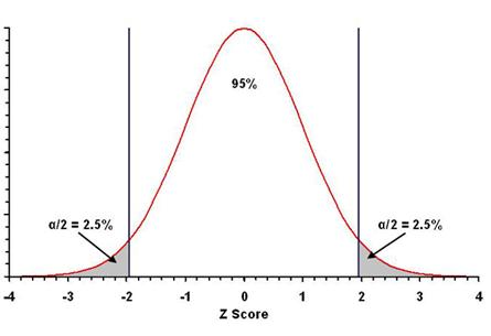
¨  Since values either too small or too large should lead to rejection of the null hypothesis, we need to find the “low” critical value with 47.5% of the values between it and the mean, and we need to find the “high” critical value with 47.5% of the values between it and the mean (47.5% + 47.5% = 95% total).

¨  This means that for a non-directional (two-tailed) hypothesis test, the error probability is divided between the two sides of the distribution, α/2 = 0.05/2 = 0.025 on each side, for a total error probability of α/2 + α/2 = 0.025 + 0.025 = 0.05, or 5%.

¨  For the normal distribution (Z-scores), the values encompassing 95% of the statistical values on either side of the mean are –1.96 and +1.96, as noted in Topic 5 for a 95% confidence interval (use Table A.1 or Excel file).

·       What are the two-tailed critical values in the normal distribution for α = 0.10, 0.02, and 0.01?

¨  As seen in the figure above (and Figure 8.1 in the text), the critical values that result in a rejection of the null hypothesis (–1.96 and +1.96) are in both tails of the distribution. Hence, it is a two-tailed test.

n   One-tailed tests are used for directional hypotheses.

¨  For mean differences, the test of a directional hypothesis determines whether one mean is either higher or it is lower than the other; the direction of the test (high or low) is stated in the hypothesis.

¨  The total α (type I error probability) is 0.05. Thus, we need to find the critical value below which lies 95% of the statistical values on only one side of the mean. Any observed value that exceeds that value in the hypothesized direction leads to rejection of the null hypothesis.

·       This region (gray in the figure below if one mean is thought to be higher than the other) is the rejection zone.

·       Observed values in this zone leads to rejection of the null hypothesis.

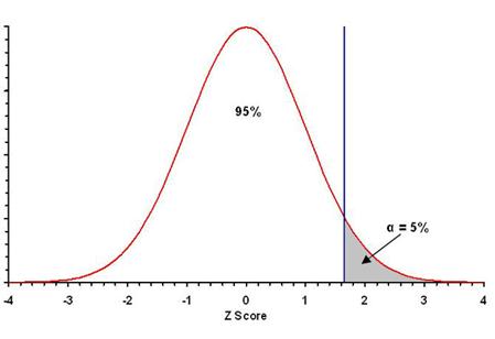
¨  Observations on only one side of the distribution lead to rejection of the null hypothesis. If one mean is thought to be larger than the other, then we need to find the critical value on the positive side of the distribution with 95% of the values less than it (95% total).

¨  The rejection area is on only one side of the distribution, α = 0.05 on the “high” side, for a total error probability of 0.05, or 5%.

¨  For the normal distriubtion (Z-scores), the value with 95% of the statistical values equal to or less than it is +1.645 (use Table A.1 or Excel file).

·       What are the one-tailed critical values in the normal distribution for α = 0.10, 0.02, and 0.01?

¨  As seen in the figure above (and Figure 8.2 in the text), the values that result in a rejection of the null hypothesis (+1.645) are in one tail of the distribution. Hence, it is a one-tailed test.

n   The distinction between a one-tailed and a two-tailed hypothesis is important because:

¨  they represent different research questions, and

¨  they are tested differently.

n   As a general rule, one-tailed tests are preferred unless the literature and logic provide no reason or rationale why effects would be in which direction or the other.

¨  Don’t use the wrong test for your hypothesis.

¨  Conduct a thorough search of the existing literature when developing your research question and hypothesis.

Click to go to the next section (Section 8.3)