PEP 6305 Measurement in
Health & Physical Education
Topic 8:
Hypothesis Testing
Section 8.3
 Click to go to
back to the previous section (Section 8.2)
Click to go to
back to the previous section (Section 8.2)
Power and Sample Size (pp.
166-170)
n
Power refers to the ability of a statistical test to detect
an effect of a certain size, if the effect really exists.
¨
This is the same as saying that power is the probability of
correctly rejecting a false null hypothesis.
¨
Power is related to
type II error (β): Power = 1 – β.
¨
Power increases with sample size; a larger sample is more likely
to detect a real effect, and can detect smaller effect sizes.
¨
Power is higher for a one-tailed hypothesis than for the
complimentary two-tailed hypothesis, because the critical value for one-tailed
tests is lower (see the
Type I and Type II
Errors section above), and are thus “easier to reach.”
¨
Power increases as α increases, because, for example, the critical
value for α = 0.05 is lower than the critical value for α = 0.01. Hopefully the
reason why will be evident by the end of this section.
n
The following series of figures demonstrates the process of power analysis (i.e., determining the power of a
statistical test).
¨
First, determine the value of the statistic under both the null
and research hypotheses. The difference between these two is an indication of
effect size.
¨
Second, identify the distribution of the null value and the
research hypothesis value.
¨
Third, decide the values of α and β that you can live with; that
is, how important is each type of error in your study?
¨
Fourth, determine the critical value for rejecting the null
hypothesis.
¨
Fifth, determine what percent of scores are below (less than) that
same critical
value for the research hypothesis distribution. That percent is β (type
II error).
¨
Sixth, 1 – β is the power of the test; power tells you how often you will
correctly reject a null hypothesis when it is actually false. (If
it is actually true, power tells you nothing.)
n
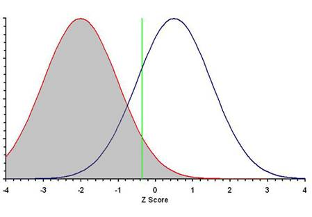
The red curve on the left
represents the sampling distribution of the null
hypothesis value, which in this example is Z = –2. Sampling error
results in the range of values on either side of the population mean Z = –2.

n
The blue curve on the
right represents the sampling distribution of the
research hypothesis value, which in this example is Z = 0.5. Sampling
error results in the range of values on either side of the population mean Z =
0.5.
n
The investigator sets the values α = 0.05 and β = 0.20.
¨
The investigator decides a type I error is four times more
important than a type II error.
n
The green line shows
the critical value for an error probability α = 0.05; in this
example, the critical value is Z = –0.335. There is only one critical value.
n
If data analysis yields a value of Z < –0.335 (left of the
green line), the null hypothesis is not rejected.
¨
If the null hypothesis
is actually TRUE, the failure to reject is a correct decision,
which will occur in 95% (the area under the red curve to the left of the green
line) of samples in which the null hypothesis is actually true.
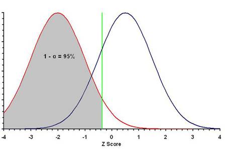
¨
If the research hypothesis
is actually TRUE (the null is FALSE), the failure to reject is
a type II error (β), which will occur in 20% (the area under the
blue curve to the left of the green line) of samples in which the null
hypothesis is actually false.
n
By contrast, if data analysis yields a value of Z ≥ –0.335 (right of the
green line), the null hypothesis is rejected.
¨
If the null hypothesis is
actually TRUE, this rejection is a type I error (α), which will occur
in 5% (under the red curve to the right of the green line) of samples in which
the null hypothesis is actually true. (Is this
a one-tailed or a two-tailed hypothesis test?)
¨
If the research hypothesis
is actually TRUE (the null is FALSE), this rejection is a
correct decision, which will occur in 80% (under the blue
curve to the right of the green line) of samples in which the null
hypothesis is actually false. The percent of scores in this region
(1 – β) is the power of the test.
n
Remember: you will never know whether the null or research
hypothesis is really true (if you did, you wouldn't need to do the experiment!).
¨
But you can estimate the probability that your decision is
right or wrong.
n
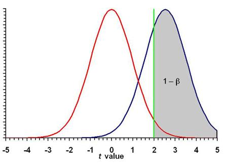
Recall that power increases as α increases. Look at
the figure just above. If the critical value (the green line) was moved to the
left, meaning that the α value (error probability) was getting larger (say from α =
0.05 to α = 0.10), then the gray shaded area representing the power of the test
also becomes larger.
¨
A higher percentage of the scores are in the gray area, which
means that power (1 – β) increases and type II error probability (β) decreases.
¨
You are more likely to reject a null hypothesis that
is in reality false; this will occur in (1 – β)% of samples.
¨
Increasing the chance of rejecting a false null hypothesis is the
key concept of statistical power.
¨
However, increasing α increases the probability of a type I error,
which means that you are more likely to reject a null hypothesis that is
really true, which is a mistake! This is the price for increasing the power of a statistical
test in a given set of data.
¨
You can have low values of both α and β but you have to
increase
the sample size substantially, which becomes expensive and time-consuming.
n
In addition to critical value (corresponding to the α value), two other factors increase power.
¨
Using a one-tailed hypothesis rather than a two-tailed hypothesis.
The one-tailed critical value is less
than the two-tailed value, so the green line
in the figure shifts to the left, thus increasing the (1 – β) shaded
area.
¨
Sample size; a larger sample shifts the entire
research hypothesis curve to the right
(critical value remains the same),
thus increasing the (1 – β) shaded area, because a larger sample results in a
smaller standard error, which is used to compute the observed statistical value.
This effect is demonstrated in the next section.
Sample Size
n
An example for computing sample size for a t test is given
in the textbook (pp. 169-170).
n
Essentially, to estimate the sample size needed for a study, you
run the statistical analyses “in reverse,” starting with the size of the effect,
specifying the error probabilities, and then solving for N.
n
While conceptually
simple, estimating sample size can be complex and tedious; I recommend enrolling
in higher-level statistics courses if you want to learn the mechanics in detail.
n
For the purposes of this course, I would like you to understand
how sample size is related to power in a general sense.
¨
When you need to compute sample size (e.g., for your thesis), your understanding of the concept will be useful to you
and whomever you consult for assistance.
n
Power is a function of the effect size and degrees of freedom.
¨
Power = effect size × df (this is the concept; this is
not an
actual formula for power)
n
If effect size, df, or both are increased, power increases.
n
The concept of effect size was discussed in the
previous section.
 ¨
A larger effect size is easier to detect, so a larger effect size increases
statistical power.
¨
A larger effect size is easier to detect, so a larger effect size increases
statistical power.
n
The concept of degrees of freedom (df) was introduced in
Topic 4.
¨
df are required to compute and interpret statistical values.
¨
The df of a statistic determine the sampling distribution of that
statistic.
¨
df are a function of sample size (N): larger N = larger df.
n
You can solve for sample size by rearranging the terms in a power
equation:
¨
Power = effect size × df, so
¨
df = power / effect size
¨
And since df depends on N (sample size), if you know df you can solve for N
n
We will demonstrate the effect of sample size using the data for
the example shown in Figure 10.1 in the text.
¨
The sample size is N = 100 (n = 50 subjects in each group).
¨
The red curve on the left
is the null hypothesis, and the
blue curve on the right is the
research hypothesis.
¨
The green line is the
critical value for rejecting the null
hypothesis.
¨
In this two-tailed test, the type I error probability is split
into each tail, with the total α = 0.05.

¨
The type II error probability is β = 0.295.

¨
The power is (1 – β) × 100% = (1 – 0.295) × 100% = (0.705) × 100%
= 70.5%.
¨
Thus, you will correctly reject a false null hypothesis in about 7
of 10 samples.
¨
A generally accepted minimum for power is 80%.
¨
How many subjects would we need to have a power of 80% for the
effect specified in the research hypothesis?
¨
The answer (which you can compute using the method in the text) is
N = 126 (n = 63 in each group).

¨
The dashed blue curve is the research hypothesis if N = 100. The
solid blue curve is the research hypothesis if N = 126.
·
The critical value is
essentially unchanged (Why?).
·
The solid blue curve (N = 126) is to the right of the
dashed blue curve (N = 100).
·
80% of the research hypothesis values
now lies to the right of the critical
value.
·
Power increased from 70% to 80% just by increasing the sample
size. (What is the type I error probability?)
¨
The determination of sample size should occur before the
study begins to ensure you have sufficient statistical power in your data to
detect the effect stated in the research hypothesis.
Formative
Evaluation
n
I asked many questions through the course of this Topic. Make sure
you know the answers to all of them.
You have reached the end of Topic 8.
Make sure to work through the Formative Evaluation
above and the textbook problems (end of the chapter).
(remember how to enter data into R Commander?)
You must complete the review quiz (in the Quizzes
folder on the Blackboard course home page) before you can advance to the next topic.


