PEP 6305 Measurement in Health & Physical Education

Topic 8: Hypothesis Testing

Section 8.1

n   This Topic has 3 Sections.

Reading

n   Vincent & Weir, Statistics in Kinesiology, 4th ed. Chapter 10 “The t Test: Comparing Means from Two Sets of Data”

Objective

n   This topic introduces the basic concepts of hypothesis testing.

n   It is more important to understand these concepts than to memorize the formulas and application of t tests.

¨  t tests, the focus of the chapter, are conceptually similar to Z-tests, except the statistic (t) is compared to the t distribution instead of comparing Z to the normal distribution.

¨  The t distribution is similar the normal distribution, except for an adjustment for samples with N < 120.

¨  Any hypothesis that can be tested with a t test can also be tested with analysis of variance (ANOVA), which is our next Topic (ANOVA and t test conclusions will always be exactly the same). ANOVA is more general than t tests because ANOVA can test a variety of other hypotheses.

¨  You can compare two groups (independent t test) or compare two measures in one group (paired t test) in R Commander, under Statistics>Means>Independent samples t-test... See the R Help menus for instructions.

Note

n   This topic is fairly long and detailed; please allow yourself sufficient time to study and complete it.

Overview: Research Hypothesis vs. Null Hypothesis

n   Recall from Topic 1 that a research hypothesis is a potential answer to a research question about a well-defined problem.

¨  The research hypothesis is developed from a thorough review of the literature; it is not “a guess.”

·       Ideally, the research hypothesis states the direction (see the Two-Tailed and One-Tailed Tests in the following section) and the size (see the Effect Size in the following section) of the hypothetical effect.

¨  The research hypothesis is not tested by statistical analysis. Statistical analyses test the null hypothesis.

¨  The null hypothesis is written so that if it is true then the research hypothesis cannot also be true.

·       The null hypothesis directly contradicts the research hypothesis. Both hypotheses cannot be true.

·       Data that show that the null hypothesis is probably false (see the Type I and Type II Errors in the following section), support (do not "prove") the research hypothesis.

¨  For example, you compare a treatment group to a non-treatment (control) group. The research hypothesis is that the treatment will improve outcome in the treatment group. The null hypothesis is that the treatment group will have the same or worse outcome as the control group.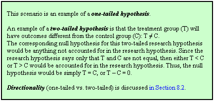

·       In symbolic terms, for this example the research hypothesis is: Treatment (T) – Control (C) > 0, or T – C > 0. The outcomes in T will be higher (better) than the outcomes in C. If we rearrange the terms so that T is on the left of the greater than sign (add C to the right-hand side), then T > C is another way to state the research hypothesis.

·       The null hypothesis is: T – C ≤ 0. The null hypothesis has to account for everything not accounted for in the research hypothesis. Since the research hypothesis is T > C, the null hypothesis has to account for both T = C and T < C. Thus, T ≤ C.

·       The statements T > C and T ≤ C cannot both be true. T must either “greater than” or “less than or equal” to C.

·       If a statistical test shows a low error probability (p ≤ 0.05) assuming that T ≤ C (the null hypothesis) is true, then T > C (the research hypothesis) is more likely to be correct and is thus supported.

·       If a statistical test shows a high error probability (p > 0.05) assuming that T ≤ C (the null hypothesis) is true, then T > C  (the research hypothesis) is less likely to be correct and is thus not supported.

·       Suppose a statistical test of the data show that the error probability of the null hypothesis is p = 0.009; this means that the groups are likely to actually have different outcomes.

·       You conclude that the evidence supports the research hypothesis (treatment improves outcomes).

n   The null hypothesis is tested by comparing an observed value (computed from sample data) to a statistical distribution.

¨  The investigator designs a study to manipulate the conditions in order to produce data (evidence) to support the research hypothesis.

¨  The investigator then collects data and computes a statistical value. This value is the observed value of the statistic.

¨  The investigator identifies the statistical distribution that provides the sampling distribution of the statistic if the null hypothesis is true.

¨  The observed statistical value is compared to the statistical distribution to determine what percent of values are more extreme than the observed value (see the Two-Tailed and One-Tailed Tests in the following section).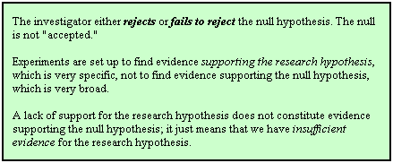

¨  If the error probability of the observed value is low (<0.05), then the conclusion is that the investigator changed the conditions “significantly”. The null hypothesis is rejected, providing support for the research hypothesis since it is a more likely explanation for the data than the null.

·       What is the conclusion if the null hypothesis is not rejected?

·       The decision to reject or not reject the null hypothesis can never be made with certainty, although the probability of making an incorrect decision can be estimated (see the Type I and Type II Errors and the Power and Sample Size in the following sections).

n   Maybe another example would be useful? After reviewing the literature, an investigator states this research hypothesis: Daily aerobic exercise changes serum cholesterol level. The null hypothesis is that daily aerobic exercise has no effect on serum cholesterol.

¨  The investigator measures serum cholesterol in a sample of subjects; the mean serum cholesterol is the same in both groups.

¨  The investigator randomly assigns the subjects to two groups.

¨  The first group receives a treatment: aerobic activity for 30 minutes per day for six weeks. The second group receives no treatment.

·       Treatment (exercise or nothing) is the condition manipulated by the investigator (it is the independent variable). No other condition is manipulated (all other conditions are the same).

¨  At the end of six weeks, the investigator again measures serum cholesterol.

¨  The investigator computes a statistical value from the data (such as to compare the change over time between groups).

¨  The observed value is compared to the distribution of that statistic which would occur if the serum cholesterol were equal in both groups.

¨  This comparison shows that the observed statistical value is found to have an error probability of 0.003, which is <0.05.

·       The observed value would only occur 3 times in 1000 such studies if serum cholesterol were really equal in both groups.

¨  The investigator rejects the null hypothesis.

·       It is more likely that the serum cholesterol levels in the groups differed.

¨  The analysis thus supports the research hypothesis that daily aerobic exercise changes serum cholesterol.

·       Aerobic exercise must have affected serum cholesterol because the subjects were randomly selected and randomly assigned to groups, and all other conditions during the study were the same for all subjects in both groups.

n   Let's discuss the concepts underlying hypothesis testing in more detail...

Click to go to the next section (Section 8.2)