PEP 6305 Measurement in
Health & Physical Education
Topic 10:
Repeated Measures
Section 10.2
 Click to go to
back to the previous section (Section 10.1)
Click to go to
back to the previous section (Section 10.1)
Repeated Measures
ANOVA in R Commander
n
Vincent demonstrates the raw score method to calculate F
for repeated measures ANOVA.
¨
We will not review the raw score method because you will probably
(hopefully) never calculate ANOVA by hand.
¨
You can also compute the F value by entering the data into
the formulas shown
in the previous section, as we
reviewed with simple ANOVA.
¨
We will review how to do repeated measures ANOVA in R Commander. Use
R Commander to complete the assignment and exam.
n
The null hypothesis is that the means of all of the measures are
equivalent. What is the
research hypothesis?
n
As an example, we'll use the data shown in textbook Table 12.1:
n
Computer output for repeated measures ANOVA can be used to make an ANOVA
table that shows all of the sources of variation:

n
For the data in Table 12.1, the ANOVA table is:

Let's see how to make this table using the output from R Commander.
n
R
Commander
¨
Download
the 'Table12.1' data file from Blackboard, or ight-click and "Save target as..." to download and save the
dataset Table12.1 to your computer.
Open R Commander and load the Table12.1 dataset. Click on the 'View data set'
button to see the data layout.
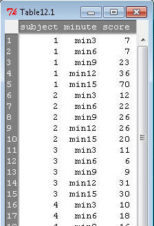
¨
Notice that the data are entered so that each subject has multiple
rows, one row for each repeated measure. The column labeled 'subject' has the
subject number. The second column labeled 'minute' has the measure name or
number. In this example, the data were collected at minutes 3, 6, 9, 12, and 15.
The third column has the score for the particular subject and measure. This
data set-up is different from a non-repeated measures study: it's important to
set the data up correctly for the analysis you're doing when entering your own
data. For repeated measures in R Commander using the below method,
you need multiple rows per subject (one row for each measure. (this is not
always true in other statistical programs, so you need to check how to enter the
data for repeated measures if you use a different program)
¨
Load the ez
package in R Commander.
¨
Here is the command you'll type in the R
Commander Script Window to do the ANOVA described above:
ezANOVA(data=Table12.1, dv=.(score), wid=.(subject), within=.(minute),
detailed=TRUE)
¨
What does all of that mean? As before, ezANOVA
is the name of the program, and the rest in the parantheses is the program
input/information that the program needs to run the analysis. The
ezANOVA program needs the following information
for one-way repeated measures (within-subjects) ANOVA:
¨
data=Table12.1
tells the program to use the Table12.1 dataset.
¨ dv=.(score)
tells the program that the dependent variable
(dv)
is the variable called 'score'.
¨
wid=.(subject)
tells the program which variable (subject) identifies the subjects.
¨ within=.(minute) tells the
program which variable (minute)
identifies the index for the repeated measures; measure is a within-subjects factor because each
subject was measured multiple times.
¨ detailed=TRUE tells the program to print out a little more information
than the default output, including the SS values.
¨
Once you've typed in the command shown above, click the Submit button to the
lower right of the Script Window, and you should see some Output:
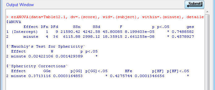
n
All of the information needed to create the ANOVA table above is present in this
output. The SS value for the "Intercept" effect denominator (SSd)
is what is labeled "Between Subjects" SS in the above table. The SS value for
the "minute" effect numerator (SSn) is the "Between Measures" SS in the above
table, and the minute effect SSd is the "Error" SS in the above table. The MS
values for the table can be computed by dividing each SS by its respective df,
and the F values by dividing the appropriate MS values.
n
Post hoc tests are performed only after the ANOVA F test indicates
that significant differences exist among the measures.
¨
If the F test is not significant, post hoc tests are
inappropriate.
¨
To
see a plot of the means for each minute, type (or copy and paste) the following
text into the R Commander Script window and click Submit:
ezPlot(data=Table12.1, dv=.(score), wid=.(subject), within=.(minute),
x=.(minute),
levels=list(minute=(list(new_order=c('min3','min6','min9','min12','min15')))))
Post Hoc
Tests
n
Similar to simple
ANOVA, post hoc statistical tests can be done to identify which
measures differ from one another.
n
Post hoc tests are performed only after the ANOVA F test indicates
that significant differences exist among the measures.
¨
If the F test is not significant, post hoc tests are
inappropriate.
n
The Scheffé interval and Tukey HSD, discussed in
Topic 9, can be used to compare
and interpret differences among the repeated measures in the same way as
comparing groups in simple ANOVA.
¨
Substitute the number of repeated measures instead of
the number of groups, and n has the same value for all measures
(i.e., the total N).
n
Scheffé Interval

Tukey HSD

Adjustments for
Violations of Sphericity
n
The text presents two methods to use if there is evidence that
sphericity may not be present.
¨
Violation of the sphericity assumption increases the
type I
error probability.
¨
The two methods include adjustments to ensure that the type I
error probability is maintained at the specified level.
¨
Both methods adjust the df of the measures MS and the df of the
error/residual MS to accomplish the correction.
n
The Greenhouse-Geisser adjustment is simple, but
over-corrects in many instances, thus making the type I error probability
too small.
n
The Huynh-Feldt adjustment is a more moderate adjustment.
n
These adjustments are only relevant if the unadjusted F
value is statistically significant, because the adjustments always increase
the p value—if it is already >0.05, then increasing it would not change your
decision (which is to not reject the null hypothesis).
n
The computation of these adjustments requires computing all of the
variances and covariances for the residuals, so we will not review them here.
n
Most advanced statistics programs automatically include
these adjustments in their repeated measures output.
In the R Commander output, you
can find the result of Mauchly's test for sphericity (if p<0.05 for Mauchly's
test, then the assumption is
likely violated), and the Greenhouse-Geisser (GG) and Huynh-Feldt (HF) adjusted
p-values for the repeated effect. NOTE: these corrections are
only printed and only needed when there are at least 3 repeated measures; there
is no way to violate sphericity with only two measures.
Formative
Evaluation
n
Use R Commander to work the two problems at the end of the chapter
(you don't have to do the post hoc tests, parts f and g of Problem 1).
You have reached the end of Topic
10.
Make sure to work through the Formative Evaluation
above and the textbook problems (end of the chapter).
(remember how to enter data into R Commander?)
You must complete the review quiz (in the Quizzes
folder on the WebCT course home page) before you can advance to the next topic.