PEP 6305 Measurement in
Health & Physical Education
Topic 7:
Regression
Section 7.1
n
This Topic has 2 Sections.
Reading
n
Vincent & Weir, Statistics in Kinesiology, 4th ed. Chapter
8 “Correlation
and
Bivariate Regression” pp. 116-132 and Chapter 9 "Multiple Correlation and
Multiple Regression"
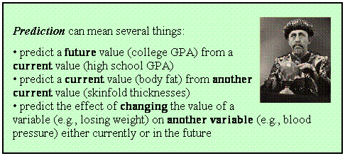
Purpose
n
To discuss and demonstrate the concepts and application of simple
(bivariate) and multiple (multivariate) regression.
Simple
(Bivariate) Regression
 n
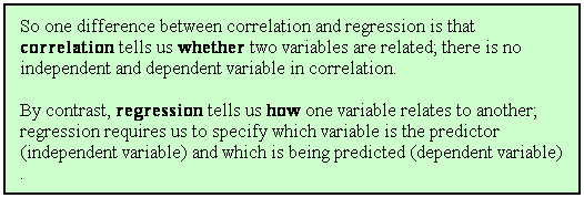
Correlation tells us only if two variables are related. What if we
want to predict or estimate the value of one variable using the value of another
variable?
n
Correlation tells us only if two variables are related. What if we
want to predict or estimate the value of one variable using the value of another
variable?
¨
Such as using high school grade point average predict (to some degree)
college freshman year grades.
n
Regression is a statistical technique that allows us to predict
the value of one variable using the value of another variable.
¨
The variable being predicted is the dependent variable; its
value depends on the value of the other variable.
¨
The variable used to make the prediction is the independent
variable; its value does not depend on (it is
independent of) the value of the other variable.
 ¨
For example, we may want to predict VO2max (aerobic
fitness) from 1.5 mile run times, because 1.5 mile run times are easier to measure
compared to doing a full maximum-effort test and measuring VO2 using
a metabolic cart in a laboratory.
¨
For example, we may want to predict VO2max (aerobic
fitness) from 1.5 mile run times, because 1.5 mile run times are easier to measure
compared to doing a full maximum-effort test and measuring VO2 using
a metabolic cart in a laboratory.
¨
Is VO2max in this example the independent or
dependent variable?
n
Regression computes an equation for the
line of best fit,
which is also called the regression line.
¨
The equation is similar to the one for a line, which
(remember algebra class?) is Y = bX + c, where
b is
the slope of the line and c is the intercept, or the
point where the line crosses the Y axis
(in other words, where X = 0).
¨
Simple regression analysis computes the values for b and
c
using the following formulas:
 Thus,
b is the product of the correlation coefficient (r) and the ratio
of the SD of Y to the SD of X.
Thus,
b is the product of the correlation coefficient (r) and the ratio
of the SD of Y to the SD of X.
 ,
which is the same as
,
which is the same as  .
.
¨
Look closely
at these formulas. If b = 0, what is the value of c? What is the correlation of X
and Y if b = 0? (Answers)
n
With the computed b and c values, you can predict values of Y
from particular values of X.
¨
The difference between a subject’s predicted score and a person’s
actual (observed) score on the dependent variable is that subject's prediction error, also called the
residual.
¨
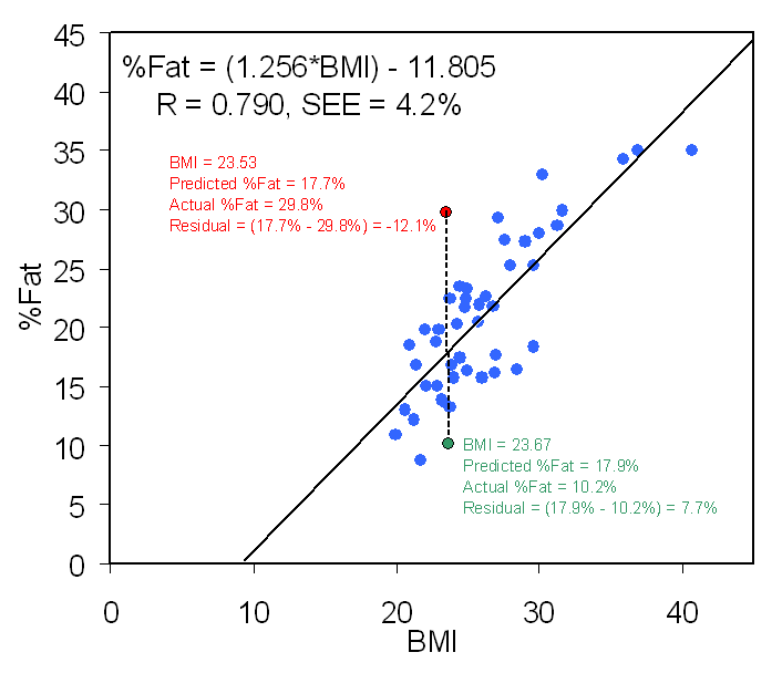
Figure 8.6 in the text and the figure below
show these components:
¨
Y is %Fat (percent body fat) and X is BMI (body mass
index). The mean of %Fat is 20.823% and the SD is
6.809%. The mean of BMI is 25.978 and the SD is 4.284.
¨
The correlation between %Fat and BMI is r = 0.790, a
relatively
large, positive association.
¨
The slope of the line of best fit (b) is 1.256. [from
the formula above: b =
0.790*(6.809/4.284) = 0.790*1.589 = 1.256 ]
¨
The intercept (c) is -11.805. [from the formula: c = -bX + Y = -(1.256*25.978) +
20.823 = -32.628 + 20.823 = -11.805 ]
¨
The predicted values (not shown) all lie directly on the regression line.
¨
The residuals (errors of prediction) are the vertical
distances from the regression line to the data points.
¨
For example, in the figure at the left, the subject represented by the
red point has a BMI of 23.53 and a
predicted %Fat of 17.7%, but their actual %Fat is 29.8%; thus, the
residual for this subject = actual - predicted = 17.7% - 29.8% = -12.1%. The
regression equation
underestimates their %Fat by 12.1%.
¨
By contrast, the subject represented by the
green point has a BMI of 23.67 and a
predicted %Fat of 17.9%, which is almost the same as the predicted value for
the red point because the BMI values are almost the same. However, the subject
at the green point has an actual %Fat of only 10.2%, which means that
their residual is 7.7%. The regression equation overestimates their %Fat by 7.7%.
¨
The equation overestimates %Fat for some subjects and
overestimates it for other subjects. So how do we know how precise the
estimation is?
n
The standard error of the estimate (SEE;
the population value is represented by σres) is the
square root of the average of the squared residuals (why
square the residuals for the average?), which can be said to be the SD of the residuals.
 where
where
 (called
“Y-hat”) is the symbol for the predicted Y value.
(called
“Y-hat”) is the symbol for the predicted Y value.
n
An easier formula is:
 which
requires only the SD of Y and the squared correlation coefficient (r2) between X
and Y.
which
requires only the SD of Y and the squared correlation coefficient (r2) between X
and Y.
n
The second formula shows that the precision of the estimate depends on
the magnitude of the correlation between the independent and dependent
variables. As the correlation increases, the SEE becomes smaller (relative to the
SD of Y).
¨
The SEE can be interpreted as the size of the average
residual (on either side of the line of best fit).
¨
The SEE is
normally distributed, so we can create a
95%
confidence interval (CI) for the predicted value: 95% CI = 1.96*SEE.
¨
For example, when BMI is used to predict %Fat, 95 times out of 100 the actual
value will be within ±(1.96*SEE) of the predicted value. For the sample data in
the graph above, the 95% CI = (1.96*4.2%) = 8.2%. So, 95 times out of 100,
actual %Fat will be within ±8.2% of the value predicted from BMI using this
equation. So, for the predicted value of the red point the 95% CI for the
predicted value (the value on the line) is 17.7% ± 8.2% = 9.5% to 25.9%. What is the 95% CI for the
predicted value of the
green point? (Answer)
¨
Notice that the actual value for the
red point
lies
outside
the 95% CI, whereas the actual value for the
green point
lies
within the
95% CI. This can be seen in the graph above; the red point
lies somewhat outside the "cluster" of its fellow data points, whereas the
green point is more a part of the crowd.
The regression equation "works better" (smaller prediction error or residual)
for
green than for red.
¨
Unless the correlation is perfect (r = 1.00 or r
= –1.00),
there will always be some error in prediction. Hence, the predicted values will
always differ from the actual values. The idea is to get the
difference as small as possible.
n
The SEE should be relatively small and the cost of measuring the
independent variable should be small compared to measuring the dependent
variable, otherwise it wouldn’t be worth using the regression equation (because
it would be imprecise, costly, or both).
n
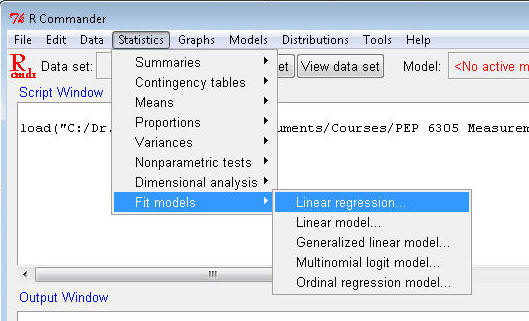
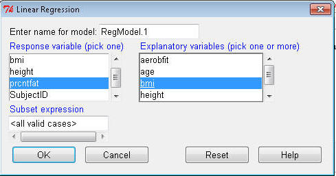
Open R Commander and load Dataset6305.
¨
Select Statistics>Fit models>Linear regression...
¨
Highlight prcntfat in the Response (dependent) variable box;
highlight bmi in the Independent(s) box. Click OK.
¨
The output file contains several pieces of information:
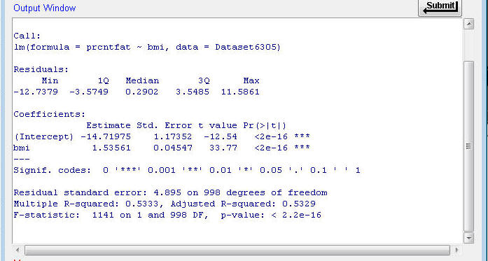
¨
The Coefficients part
gives you the regression equation results. The column labeled “Estimate” in this table shows the regression weight
(the b value) for bmi (b = 1.53561) and the intercept for the regression equation (c = -14.71975).
¨
The value of b for BMI indicates that body fat increases by
approximately 1.54% for
every point that BMI increases.
¨
The fourth and fifth columns provide a statistic (t-value) and the
respective error probability for testing whether b = 0. The error probability for
b = 0 is p < 0.001 (in fact, WAY below 0.001). Thus, the values of b differs from 0 by
more than what would be expected from sampling error alone in this sample.
¨
The bottom part of the output shows you the R-squared value and the
error probability (p-value) that the amount of variation
in prcntfat that is predicted by BMI is equal to 0. The p-value for the error probability is p < 0.001 (it's
actually 2.2 x 10⁻¹⁶, which is a very small value, much less than
0.001). This means that the value of R2
(0.5333) is very unlikely to have occurred if the true value in the
population is R2 = 0. Consequently, we can say that BMI is a
statistically significant predictor of prcntfat.
¨
The Standard Error of Estimate (SEE)
is reported as the 'Residual standard error' and the“adjusted” R2
value that is used when there are several independent variables.
¨
Using the SEE, what is the
95% CI for the prediction of prcntfat
from BMI in your data?
 Click
to go to the next section (Section 7.2)
Click
to go to the next section (Section 7.2)