PEP 6305 Measurement in Health & Physical Education
Topic 11: Reliability
Section 11.2
![]() Click to go to
back to the previous section (Section 11.1)
Click to go to
back to the previous section (Section 11.1)
Intraclass Correlation
n The method that we will use to compute a reliability estimate is called intraclass correlation.
¨ Intraclass correlation uses the MS values that are computed by analysis of variance (ANOVA).
n Intraclass correlation can be computed using one-way (simple) ANOVA or two-way (repeated measures) ANOVA. The two-way ANOVA will be used in this course.
¨ The one-way ANOVA model is used if differences between the repeated measures are considered to be error--contrary to intuition, this is not always the case.
¨ If the F test of the repeated measures effect is not significant, the difference in reliability estimates between the one-way and two-way models is negligible.
¨ You will not be asked to compute reliability using one-way ANOVA in this course.
n Calculating reliability is tedious to do manually, but is quite easy with a program such as LazStats. The approach in this topic will be to use LazStats to calculate ANOVA and illustrate the sources of the data.
n Reliability Example 1 – Random Numbers
¨ This example uses a 4-trial fictional test administered to 7 fictional individuals. The test scores are random numbers, so the reliability should be approximately 0.

¨ The data set consists of a total of 28 scores, 7 subjects and 4 trials (7 x 4 = 28).
¨ Intraclass reliability will be illustrated using (two-way) repeated measures ANOVA of the 28 scores. Here is the resulting ANOVA table:

¨ The F value of 0.95 (p = 0.437) is very low, showing that the variance among the four trials is caused by chance variation: the trials do not differ.
¨ One equation for calculating intraclass reliability (Rxx) from a two-way ANOVA is:
Rxx = (MS People - MS Residual) / MS People = (4.57 - 2.85)/4.56 = 1.72/4.56 = 0.377
(this Rxx is the same as the intraclass correlation coefficient R2 described by Vincent & Weir, p. 218, Table 13.4 Model 3,k--it includes only random error, the MS Residual, and does not include trial-to-trial differences, the MS Between Measures, as error. Other types of reliability include the trial-to-trial differences as error, such as when determining how closely raters agree (use Model 2,k from Table 13.4).
¨ The intraclass reliability of 0.377 is for a test score that is the mean of all 4 trials. (The effect of number of trials on test reliability is covered below.)
¨ Note, the 28 scores in this example are random numbers so the reliability estimate should be low and near 0. The reason that it is not exactly 0 is the sample size of 7 subjects is very small, so the sampling error is large. If we had a larger sample (> 50), the sampling error would be smaller and the value would likely be very close to 0.
¨ Assuming the intraclass reliability was actually 0.377, we can conclude the following:
· The proportion of total variance, measuring true individual differences in whatever was tested, was 0.377 (37.7%).
· The proportion of total variance that is measurement error is 0.623 (1.00 – 0.377 = 0.623), or 62.3%.
· Thus, measurement error is much larger than true score differences. Reliability is low, and this is a poor test.
n The purpose of this section is to illustrate the use of R Commander to estimate test reliability.
¨ This table provides actual leg strength data for a sample of 6 subjects, each tested 4 times, i.e., there were 4 trials. Download the ReliabilityEx file from Blackboard or right-click and "Save target as..." to download and save the ReliabilityEx file and import it into R Commander.

- Enter the following text into the R Commander Script window:
ezANOVA(data=ReliabilityEx, dv=.(score), wid=.(subject), within=.(trial), detailed=TRUE)
n Compare your output to the following:
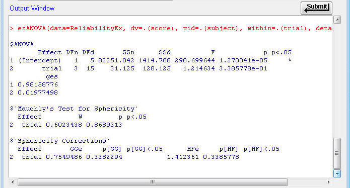
· Between Persons SS
· The SS Persons is the df for the denominator of the "Intercept" effect: SS Persons = 1414.708. The Intercept label means the variability of the subjects from the grand mean across all 4 measures.
· The MS Subjects = SS Subjects / df = 1414.708 / 5 = 282.88.
· Between Items F
· The F value for the between-trials test is 1.214624 (p = 3.385 x 10-1 = 0.339).
· Indicates that variation among the means of the four trials is within chance.
· Within People Total Variance.
· The Within Total SS is the sum of the Between Items SS (31.125) and Residual SS (128.125).
· The Residual MS = 128.125/15 = 8.542 (This is close to what you can compute to be the Total Within MS, 8.847, because the trials are not significantly different; hence, reliability estimates that do or don't consider trial to trial differences to be error would be essentially the same).
¨ Reliability Estimates
· To compute this intraclass reliability coefficient from the ANOVA table values:
Rxx = (MS Subjects - MS Residual)/ MS Subjects
= 282.88 - 8.542/282.88 = 274.338/282.88 = 0.970
· This is an intraclass reliability estimate for a score that is the sum/total of the 4 trials.
¨ Interpretation of the Reliability coefficient
· Over 97% of the variance of strength test is due to true differences in strength among the subjects – some subjects are stronger than others and the test measures these differences.
· Less than 3% of the variance of the strength test is due to random measurement error.
· We can conclude that this is a highly reliable test.
Forecasting Reliability
n The equation for forecasting test reliability with the ANOVA means squares.

n The terms are:
¨ MSP = Between People Mean Square.
¨ MSI = Residual Mean Square.
¨ k = number of trials administered.
¨ k' = number of trials for which you want to estimate reliability; this number will be either greater than or less than k, the number of trials actually measured.
n Example: An arm strength test was administered to 207 people and there were two trials, resulting in the following ANOVA table.

n Note the following information:
¨ Intraclass Reliability for two trials = 0.964 (How do we know this?)
¨ Data For Forecast Equation:
· MSP = Between People Mean Square = 1151.58.
· MSI = Residual Mean Square = 41.23
· k = number of trials administered = 2.
¨ Forecasting Reliability: For one trial (k' = 1)

¨ Interpretation - The reliability for the test if only one trial was administered would be 0.931, slightly lower than for two trials.
¨ Forecasting Reliability - For three trials (k' = 3)

¨ Interpretation - The reliability for the test if three trials were administered, the reliability would be 0.976, slightly higher than for two trials (0.964).
n Application of Forecasting
¨ The forecasting method can be used to develop a testing protocol.
¨ In the example just illustrated, the reliability of a 2-trial test was very high. This analysis showed that just using a single trial would result in only a small loss in accuracy.
¨ The method can also be used to determine how many additional trials would be required to improve reliability.
n The Spearman-Brown prophecy formula is a second method that can be used to forecast test reliability.
¨ This method estimates the increase in test reliability for a test that has been lengthened by k times (k = 2, the test is twice as long, k = 0.5, the test is half as long, etc.).
¨ The reliability of test can be estimated for a longer test. The Spearman-Brown equation is:
 where
r1,1 is the computed reliability of the test, k is times the test is
lengthened, and rkk is the estimated reliability for the test
lengthened k times.
where
r1,1 is the computed reliability of the test, k is times the test is
lengthened, and rkk is the estimated reliability for the test
lengthened k times.